Open Specy App Tutorial
Win Cowger, Zacharias Steinmetz
2024-03-27
Source:vignettes/app.Rmd
app.RmdDocument Overview
This document outlines a common workflow for using the Open Specy app and highlights some topics that users are often requesting a tutorial on. If the document is followed sequentially from beginning to end, the user will have a better understanding of every procedure involved in using the Open Specy R app as a tool for interpreting spectra. It takes approximately 45 minutes to read through and follow along with this standard operating procedure the first time. Afterward, knowledgeable users should be able to thoroughly analyze spectra at an average speed of 1 min-1 or faster with the new batch and automated procedures. If you are looking for documentation about the R package please see the package vignette
Running the App
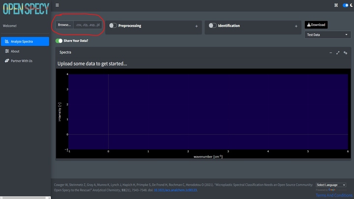
To get started with the Open Specy user interface, access https://openanalysis.org/openspecy/
or start the Shiny GUI directly from your own computer in R. If using
the package, you just need to read in the library and run the command
run_app().
run_app()Reading Data
Once the app is open, if you have your own data, click Browse at the top left hand corner of the Analyze Spectra tab.
Before uploading, indicate if you would like to share the uploaded data or not using the slider. If selected, any data uploaded to the tool will automatically be shared under CC-BY 4.0 license and will be available for researchers and other ventures to use to improve spectral analysis, build machine learning tools, etc. Some users may choose not to share if they need to keep their data private. If switched off, none of the uploaded data will be stored or shared in Open Specy.
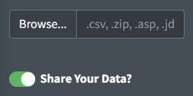
Open Specy allows for upload of native Open Specy .y(a)ml, .json, or
.rds files. In addition, .csv, .asp, .jdx, .0, .spa, .spc, and .zip
files can be imported. .zip files can either contain multiple files with
individual spectra in them of the non-zip formats or it can contain a
.hdr and .dat file that form an ENVI file for a spectral map. Open Specy
and .csv files should always load correctly but the other file types are
still in development, though most of the time these files work
perfectly. If uploading a .csv file, label the column with the
wavenumbers wavenumber and name the column with the
intensities intensity. Wavenumber units must be
cm-1. Any other columns are not used by the software. Always
keep a copy of the original file before alteration to preserve metadata
and raw data for your records.
| wavenumber | intensity |
|---|---|
| 301.040 | 26 |
| 304.632 | 50 |
| 308.221 | 48 |
| 311.810 | 45 |
| 315.398 | 46 |
| 318.983 | 42 |
It is best practice to cross check files in the proprietary software they came from and Open Specy before use in Open Specy. Due to the complexity of some proprietary file types, we haven’t been able to make them fully compatible yet. If your file is not working, please contact the administrator and share the file so that we can work on integrating it.
The specific steps to converting your instrument’s native files to .csv can be found in its software manual or you can check out Spectragryph, which supports many spectral file conversions see Spectragryph Tutorial.
If you don’t have your own data, you can use a test dataset.
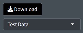
A .csv file of an HDPE Raman spectrum will download on your computer. This file can also be used as a template for formatting .csv data into an Open Specy accepted format.
Visualization
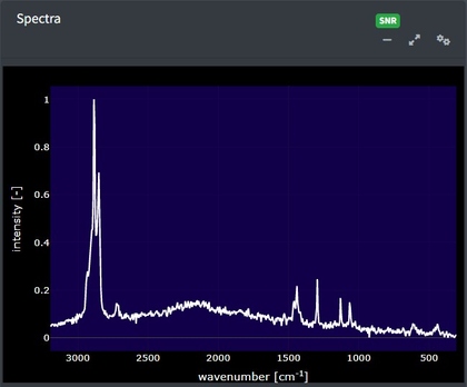
Spectra
In the app after spectral data are uploaded, it will appear in the main window. This plot is selectable, zoomable, and provides information on hover. You can also save a .png file of the plot view using the camera icon at the top right when you hover over the plot.
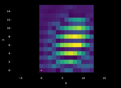
Maps
Spectral maps can also be visualized as overlaid spectra but in
addition the spatial information can be plotted as a heatmap. A similar
plot should appear in the app if you upload multiple spectra or a
spectral map. It is important to note that when multiple spectra are
uploaded in batch they are prescribed x and y
coordinates, this can be helpful for visualizing summary statistics and
navigating vast amounts of data but shouldn’t be confused with data
which actually has spatial coordinates. Hovering over the map will
reveal information about the signal and noise and correlation values.
Clicking the map will provide the selected spectrum underneath. In the
app, the colors of the heatmap are either the signal and noise or the
spectral identifications depending on whether the identification is
turned on or not. Pixels are black if the spectra does not pass the
signal-noise threshold and/or the correlation threshold.
Processing
The goal of this processing is to increase the signal to noise ratio (S/N) without distorting the shape or relative size of the peaks. After uploading data, you can process the data using intensity adjustment, baseline subtraction, smoothing, flattening, and range selection and save your processed data. Once the process button is selected the default processing will initiate. This is an absolute derivative transformation, it is kind of magic, it does something similar to smoothing, baseline subtraction, and intensity correction simultaneously and really quickly. By clicking processing you should see the spectrum update with the processed spectra.
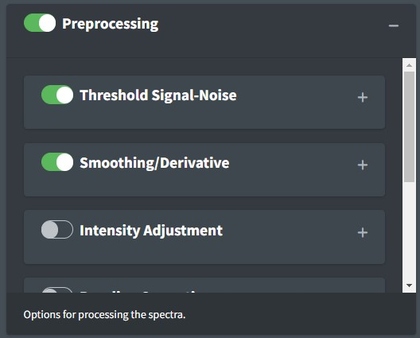
To view the raw data again, just deselect processing. Toggling processing on and off can help you to make sure that the spectra are processed correctly.
Threshold Signal-Noise
Considering whether you have enough signal to analyze spectra is important. Classical spectroscopy would recommend your highest peak to be at least 10 times the baseline of your processed spectra before you begin analysis. If your spectra is below that threshold, you may want to consider recollecting it. In practice, we are rarely able to collect spectra of that good quality and more often use 5. The Signal Over Noise technique searches your spectra for high and low regions and conducts division on them to derive the signal to noise ratio. Signal Times Noise multiplies the mean signal by the standard deviation of the signal and Total Signal sums the intensities. The latter can be really useful for thresholding spectral maps to identify particles which we will discuss later.
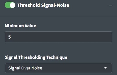
If analyzing spectra in batch, we recommend looking at the heatmap and optimizing the percent of spectra that are above your signal to noise threshold to determine the correct settings instead of looking through spectra individually. Good Signal tells you what percent of your data are above your signal threshold.

Intensity Adjustment
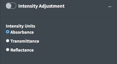
Open Specy assumes that intensity units are in absorbance units but Open Specy can adjust reflectance or transmittance spectra to absorbance units using this selection. The transmittance adjustment uses the \(\log_{10} 1/T\) calculation which does not correct for system or particle characteristics. The reflectance adjustment use the Kubelka-Munk equation \(\frac{(1-R)^2}{2R}\). If none is selected, Open Specy assumes that the uploaded data is an absorbance spectrum and does not apply an adjustment.
Conforming
Conforming spectra is essential before comparing to a reference library and can be useful for summarizing data when you don’t need it to be highly resolved spectrally. In the app, conforming happens behind the scenes without any user input to make sure that the spectra the user uploads and the library spectra will be compatible. We set the spectral resolution to 8 because this tends to be pretty good for a lot of applications and is in between 4 and 8 which are commonly used wavenumber resolutions.
Smoothing
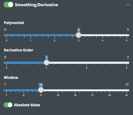
The value on the slider is the polynomial order of the Savitzky-Golay (SG) filter. Higher numbers lead to more wiggly fits and thus less smooth, lower numbers lead to more smooth fits. The SG filter is fit to a moving window of 11 data points by default where the center point in the window is replaced with the polynomial estimate. Larger windows will produce smoother fits. The derivative order is set to 1 by default which transforms the spectra to their first derivative. A zero order derivative will have no derivative transformation. When smoothing is done well, peak shapes and relative heights should not change. The absolute value is primarily useful for first derivative spectra where the absolute value results in an absorbance-like spectrum which is why we set it as the default.
Baseline Correction
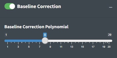
The goal of baseline correction is to get all non-peak regions of the spectra to zero absorbance. The higher the polynomial order, the more wiggly the fit to the baseline. If the baseline is not very wiggly, a more wiggly fit could remove peaks which is not desired. The baseline correction algorithm used in Open Specy is called “iModPolyfit” (Zhao et al. 2007). This algorithm iteratively fits polynomial equations of the specified order to the whole spectrum. During the first fit iteration, peak regions will often be above the baseline fit. The data in the peak region is removed from the fit to make sure that the baseline is less likely to fit to the peaks. The iterative fitting terminates once the difference between the new and previous fit is small. An example of a good baseline fit below. For those who have been with OpenSpecy a while, you will notice the app no longer supports manual baseline correction, it was a hard choice but it just didn’t make sense to keep it now that we are moving toward high throughput automated methods. It does still exist in the R function though.
Range Selection
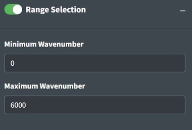
Sometimes an instrument operates with high noise at the ends of the spectrum and, a baseline fit produces distortions, or there are regions of interest for analysis. Range selection accomplishes those goals. You should look into the signal to noise ratio of your specific instrument by wavelength to determine what wavelength ranges to use. Distortions due to baseline fit can be assessed from looking at the process spectra. Additionally, you can restrict the range to examine a single peak or a subset of peaks of interests. The maximum and minimum wavenumbers will specify the range to keep in the app.
Flattening Ranges
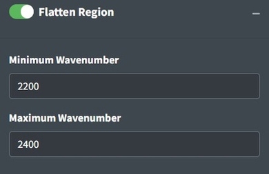
Sometimes there are peaks that really shouldn’t be in your spectra and can distort your interpretation of the spectra but you don’t necessarily want to remove the regions from the analysis because you believe those regions should be flat instead of having a peak. One way to deal with this is to replace the peak values with the mean of the values around the peak. This is the purpose of the Flatten Range. By default it is set to flatten the CO2 region for FTIR spectra because that region often needs to be flattened when atmospheric artifacts occur in spectra.
Min-Max Normalization
Min-Max normalization is used throughout the app but is not one of the options the user can specify. Often we regard spectral intensities as arbitrary and min-max normalization allows us to view spectra on the same scale without drastically distorting their shapes or relative peak intensities. In the app, it is primarily used for plotting and as a processing step before correlation analysis.

Identifying Spectra
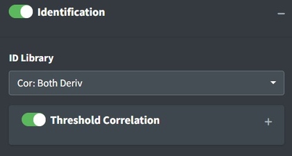
After uploading data and processing it (if desired) you can now identify the spectrum. To identify the spectrum go to the Identification box. Pro tip: if you select Identification without uploading data to the app, you’ll be able to explore the library by itself.
Reading Libraries
These options define the strategy for identification. The ID Library will inform which library is used. Both (default) will search both FTIR and Raman libraries. Deriv will search against a derivative transformed library. No Baseline will search against a baseline corrected library. This should be in line with how you choose to process your spectra. Cor options use a simple Pearson correlation search algorithm. AI is currently experimental and uses either a multinomial model or correlation on mediod spectra from the library. Correlation thresholding will set the minimum value from matching to use as a ‘positive identification’ this will black out pixels in a spectral map view if they are lower than the threshold.
Matches
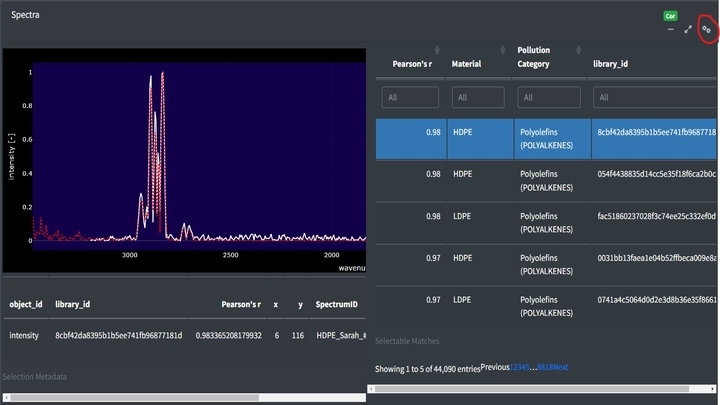
Top matches in the app can be assessed by clicking the cog in the right hand corner of the Spectra box. This will open a side window with the matches sorted from most to least similar. Clicking on rows in the table will add the selected match to the spectra viewer. Using the table’s filter options, you can restrict the range of Pearson's r values or search for specific material types.
Selection Metadata
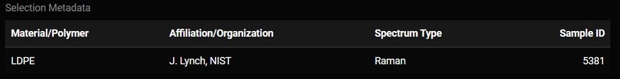
Whatever match is selected from the match table may have additional metadata about it. That metadata will be displayed below the plot. Some of this metadata may assist you in interpreting the spectra. For example, if the spectra has metadata which says it is a liquid and you are analyzing a solid particle, that spectrum may not be the best match.
Match Plot
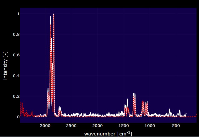
This plot is dynamically updated by selecting matches from the match table. The red spectrum is the spectrum that you selected from the reference library and the white spectrum is the spectrum that you are trying to identify. Whenever a new dataset is uploaded, the plot and data table in this tab will be updated. These plots can be saved as a .png by clicking the camera button at the top of the plot.
Characterizing Particles

Thresholding only works and shouldn’t be used for single particles. You can threshold spectral maps using the signal-noise values and/or the correlation threshold. Whatever selection you have active will inform how your spectra is thresholded. It should get thresholded in coincidence with what you see on the spectral map. Pro tip: The file that gets downloaded is an OpenSpecy with median spectra for each of your thresholded particles. You can upload that back to the app and analyze that independently.
Additional App Features
Accessibility is extremely important to us and we are making strives to improve the accessibility of Open Specy for all spectroscopists. Please reach out if you have ideas for improvement.
We added a Google translate plugin to all pages in the app so that you can easily translate the app. We know that not all languages will be fully supported but we will continue to try and improve the translations.
![]()
References
Chabuka BK, Kalivas JH (2020). “Application of a Hybrid Fusion Classification Process for Identification of Microplastics Based on Fourier Transform Infrared Spectroscopy.” Applied Spectroscopy, 74(9), 1167–1183. doi: 10.1177/0003702820923993.
Cowger W, Gray A, Christiansen SH, De Frond H, Deshpande AD, Hemabessiere L, Lee E, Mill L, et al. (2020). “Critical Review of Processing and Classification Techniques for Images and Spectra in Microplastic Research.” Applied Spectroscopy, 74(9), 989–1010. doi: 10.1177/0003702820929064.
Cowger W, Steinmetz Z, Gray A, Munno K, Lynch J, Hapich H, Primpke S, De Frond H, Rochman C, Herodotou O (2021). “Microplastic Spectral Classification Needs an Open Source Community: Open Specy to the Rescue!” Analytical Chemistry, 93(21), 7543–7548. doi: 10.1021/acs.analchem.1c00123.
Primpke S, Wirth M, Lorenz C, Gerdts G (2018). “Reference Database Design for the Automated Analysis of Microplastic Samples Based on Fourier Transform Infrared (FTIR) Spectroscopy.” Analytical and Bioanalytical Chemistry, 410(21), 5131–5141. doi: 10.1007/s00216-018-1156-x.
Renner G, Schmidt TC, Schram J (2017). “A New Chemometric Approach for Automatic Identification of Microplastics from Environmental Compartments Based on FT-IR Spectroscopy.” Analytical Chemistry, 89(22), 12045–12053. doi: 10.1021/acs.analchem.7b02472.
Savitzky A, Golay MJ (1964). “Smoothing and Differentiation of Data by Simplified Least Squares Procedures.” Analytical Chemistry, 36(8), 1627–1639.
Zhao J, Lui H, McLean DI, Zeng H (2007). “Automated Autofluorescence Background Subtraction Algorithm for Biomedical Raman Spectroscopy.” Applied Spectroscopy, 61(11), 1225–1232. doi: 10.1366/000370207782597003.